Fast AF Fourier Transform (FafFT)
I recently saw these two videos about the discrete fourier transform (DFT) and discovering the fast fourier transform (FFT) and I got re-inspired to experiment with the FFT algorithm again.
If you're not sure what a Fourier Transform is or you're not sure how the DFT or FFT algorithms work, then check out the videos above.
If you're not so keen on videos, or don't have the time, I'll try to briefly explain it.
What is the FFT?
Before covering FFT, let's first talk about what the Fourier Transform is. It takes an input from 'signal space' and converts it to 'frequency space'. What does that mean? Take a look at the following graphs
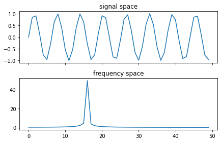
This shows a simple sine wave, and its frequency can be seen in the spike in the frequency space graph, not so interesting yet.
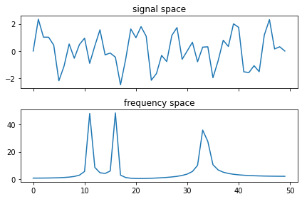
However, if we were to make our signal a bit more complex, by layering 3 different sine waves on top of each other, we see that the Fourier Transform is still able to extract the unique frequencies
There's a lot more that the Fourier Transform can do, check out the wikipedia article to learn more.
The Fast Fourier Transform is a very efficient algorithm to compute the Discrete Fourier Transform.
Wait, what is the discrete fourier transform?
I've skipped a bit about the fourier transform, but it's defined as the following complex integral.
This is a continuous operation and impractical to work with real world data in a computer. Instead, we want a version which works on discrete data.
Instead, we can turn the integral into a finite summation

and the same properties will apply. The issue with this formula is that it will have a complexity of O(n^2). This means that the run time will quadruple as the input length doubles. This is a big deal for sound processing. Typical audio is sampled at 44,100 times per second. This would need 1,944,810,000 calculations for analysing just a second of audio.
However, because of the symmetric properties of the fourier transform, there happens to be a clever trick we can do. We can split the input, apply the DFT to each half, then combine them. We can do the same trick to these smaller signals. This takes the complexity all the way down to O(n log n). This theoretically brings the calculations required for the 44100 sample signal down to ~ 680,000. That's almost 3000 times faster.
Here's what the FFT algorithm looks like written in python (using numpy)
def fft(xs):
    n = len(xs)

    # Recursion base case
    if n == 1:
        return xs

    # Split the input in half
    evens = []
    odds  = []
    for k, x in enumerate(xs):
        if k % 2 == 0:
            evens.append(x)
        else:
            odds.append(x)

    # Apply smaller FFTs
    evens = fft(evens)
    odds  = fft(odds)

    # Combine FFTs
    output = [0] * n
    for k in range(n//2):
        z = np.exp(-2j * np.pi * k / n)
        output[k]        = evens[k] + z * odds[k]
        output[k + n//2] = evens[k] - z * odds[k]

    return output
How can we speed this up some more?
As far as I am aware, there's no way to speed up the algorithm further than O(n log n), so instead, we have to use some programming optimisations.
I'm going to be writing this implementation in Rust. Don't worry too much if you're not familiar, I'll explain it as we go.
The first thing which I want to optimise is the recursion. Recursion is useful and clever and provides very simple solutions to some complex problems, but it ends up being quite slow. Every time you call a function, you push more data onto 'the stack'. The stack controls the data that you will be using regularly. This includes the input variables, any new variables you create in the function, as well as where you will return to once the function is done. This adds up quite considerably with recursive functions.
How can we possible make this non-recursive? It turns out that most simple recursive functions can be written iteratively. Let's dry run out FFT above with a small input to see what happens
- Let's take the input
[0, 1, 2, 3, 4, 5, 6, 7]withn = 8. - First, we split input in half. We get
es=[0, 2, 4, 6]andos=[1, 3, 5, 7]. - We then apply the FFT to
es.n = 4 - We split the input in half again,
[0, 4]and[2, 6]respectively. - We then apply FFT again to
[0, 4], nown = 2. - Again, we split this in half,
[0],[4]. Since these are our base cases, we can stop here. - Now that they're split, we can combine the two outputs.
Ok, let's pause here. We split the input in half 3 times before getting down to the base case, then we combine them back up again at the end. Let's try something different.
Splitting the input
Let's instead try to split up the entire input before doing any combining.
[0, 2, 4, 6], [1, 3, 5, 7][0, 4], [2, 6], [1, 5], [3, 7][0], [4], [2], [6], [1], [5], [3], [7]
We can then combine them back up just the same as before. We might notice though that we've not actually required any more space. We've just re-arranged our input. Let's zip it up back into a single array
[0, 4, 2, 6, 1, 5, 3, 7]
Much simpler. The even terms will just be moved to the left side and the odd terms will be moved to the right.
Let's take a look at what we have so far.
// This code splits the input in two
// storing the even indices in the left side of the output
// and the odd indices in the right side.
fn split_even_odd<T: Copy>(input: &[T], output: &mut [T]) {
    let n = input.len();
    let n2 = n / 2;
    for k in 0..n2 {
        output[k]      = input[k * 2];
        output[k + n2] = input[k * 2 + 1];
    }
}

// Compute the FFT over an array of complex values
// The complex type comes from num_complex
// https://docs.rs/num-complex/0.3.1/num_complex/struct.Complex.html
fn fft(mut input: Vec<Complex<f64>>) -> Vec<Complex<f64>> {
    let n = input.len();

    // Create a new array with the same length as the input
    // This will be where we store the split input
    let mut split = vec![Complex::new(0, 0); n];

    // Start with our scope over the entire array
    let mut m = n;
    while m > 1 {
        // Range over the length of the array, stepping by m each time
        // Ex: (n = 8)
        //  when m = 8, s takes on the values [0]
        //  when m = 4, s takes on the values [0, 4]
        //  when m = 2, s takes on the values [0, 2, 4, 6]
        // These values point to the start of each sub array
        // With m being the length of each sub array.
        for s in (0..n).step_by(m) {
            split_even_odd(&input[s..s+m], &mut split[s..s+m]);
        }

        // Swap the variables so that we can perform the split
        // over our new values
        swap(&mut input, &mut split);

        // Narrow the scope over which we split
        m /= 2;

        // Once m is 1, we're done
    }

    // The input variable is now split down to the base case

    // ...
}
Great! We've successfully split our input all the way down to the base case iteratively. As you can see, the implementation is already a lot more complex. That's why recursion is so nice conceptually. Anyway, let's continue.
Zipping back up
Now that we've split the input, we need to combine the values back up.
This actually follows a very similar pattern to above, we just do it backwards. So we start with m = 2 and work our way up to m = n, combining the inputs at each step. Let's see what that looks like
fn split_even_odd<T: Copy>(input: &[T], output: &mut [T]) { /* ... */ }

// Perform the combine step in-place
// This saves on us having to allocate more memory
fn combine(input: &mut [Complex<f64>]) {
    let n = input.len();
    const step: f64 = -2.0 * std::f64::consts::PI / (n as f64);

    for k in 0..n/2 {
        // This is the same as our complex exponential
        let z = Complex::from_polar(1.0, (k as f64) * step);

        // store as temporary variables since we will
        // be overwriting them next step
        let e = input[k];
        let o = input[k + n/2];

        // combine the variables above and store them as our output
        input[k]       = e + z * o;
        input[k + n/2] = e - z * o;
    }
}

fn fft(mut input: Vec<Complex<f64>>) -> Vec<Complex<f64>> {
    let n = input.len();

    // split our input all the way down
    let mut split = vec![Complex::new(0, 0); n];
    let mut m = n;
    while m > 1 {
        for s in (0..n).step_by(m) {
            split_even_odd(&input[s..s+m], &mut split[s..s+m]);
        }
        swap(&mut input, &mut split);
        m /= 2;
    }

    // combine our input all the way back up
    let mut m = 2;
    while m <= n {
        for s in (0..n).step_by(m) {
            combine(&mut input[s..s+m]);
        }

        m *= 2;
    }
}
Awesome! We've successfully removed the recursion from the FFT! This should be considerably faster. Not only as we not polluting our stack nearly as much, we're not allocating as many arrays either. Let's see where we can go from here.
Caching values
One thing you might have noticed is that we're recalculating the value z for every call to combine. This is a bit wasteful. If we can re-use those values, then we would be able to speed up our computation a bit. Starting from the m = 2 case, what values of z do we calculate?
Since k in 0..1, we get exp(-2pi * 0/m) == 1.0.
How about m = 4. This is a little more interesting, we calculate two values now, [exp(-2pi * 0/m), exp(-2pi * 1/m)] == [1.0, -i]
For m = 8. This is a little more interesting, we get [1.0, 1.41-1.41i, -i, -1.41-1.41i]. Conveniently, the values for the smaller m = 4 case are interspersed in the values for m = 8. This simplifies it a lot for us since we can calculate just a single array of our z values, and use them for all of the combine calculations.
// Perform the combine step in-place
// This saves on use having to allocate more memory
// Takes in pre-calculated z values
fn combine(zs: &[Complex<f64>], input: &mut [Complex<f64>]) {
    let n = input.len();
    let z_step = zs.len() / n;

    for k in 0..n/2 {
        let z = zs[k * z_step];

        let e = input[k];
        let o = input[k + n/2];
        input[k]       = e + z * o;
        input[k + n/2] = e - z * o;
    }
}

fn fft(mut input: Vec<Complex<f64>>) -> Vec<Complex<f64>> {
    let n = input.len();

    // split our input all the way down
    // ...

    // calculate z values
    let step = -2.0 * std::f64::consts::PI / (n as f64);
    // iterate over the range of values 0 to n/2
    // mapping every value to it's z value
    // collecting the results into a vector
    let zs: Vec<_> = (0..n/2)
        .into_iter()
        .map(|k| Complex::from_polar(1.0, (k as f64) * step))
        .collect();

    let mut m = 2;
    while m <= n {
        for s in (0..n).step_by(m) {
            // pass in pre-calculated z values
            combine(&zs, &mut input[s..s+m]);
        }

        m *= 2;
    }
}
That's better. And considerably faster. A big part of the FFT algorithm is computing those complex values, so now that we only have to do it once is a great improvement.
Now, as far as I am aware, that's as fast as we can get with the combine step. We are forced by the algorithm to make this many computations. There might be some tricks with cache lines but that's the edge of my knowledge.
However, let's look back to the splitting stage. Let's see if we can speed that up some more.
The Cherry on top
For our n = 8 example, let's see how many times we need to copy data.
input = [0, 1, 2, 3, 4, 5, 6, 7]allocate array with capacity 8copy the 8 values to [0, 2, 4, 6, 1, 3, 5, 7]copy the 8 values to [0, 4, 2, 6, 1, 5, 3, 7]copy the 8 values to [0, 4, 2, 6, 1, 5, 3, 7]
We ended up using 24 copies and allocating 8 * 2 * 64 bytes for temporary use. However, if you've been paying close attention, you might notice that the last step was useless. So we can get rid of 8 of those copies. If you've been paying really close attention, you may notice that we actually only need 2 swaps!
[0, 1, 2, 3, 4, 5, 6, 7][0, 4, 2, 3, 1, 5, 6, 7] swap(1, 4)[0, 4, 2, 6, 1, 5, 3, 7] swap(3, 6)
That's it. That's all we needed to get split our data. No allocations either.
Let's cover a bigger example. n = 16
[0, 1, 2, 3, 4, 5, 6, 7, 8, 9, 10, 11, 12, 13, 14, 15] =>
[0, 8, 4, 12, 2, 10, 6, 14, 1, 9, 5, 13, 3, 11, 7, 15]
[0, 1, 2, 3, 4, 5, 6, 7, 8, 9, 10, 11, 12, 13, 14, 15][0, 8, 2, 3, 4, 5, 6, 7, 1, 9, 10, 11, 12, 13, 14, 15] swap(1, 8)[0, 8, 4, 3, 2, 5, 6, 7, 1, 9, 10, 11, 12, 13, 14, 15] swap(2, 4)[0, 8, 4, 12, 2, 5, 6, 7, 1, 9, 10, 11, 3, 13, 14, 15] swap(3, 12)[0, 8, 4, 12, 2, 10, 6, 7, 1, 9, 5, 11, 3, 13, 14, 15] swap(5, 10)[0, 8, 4, 12, 2, 10, 6, 14, 1, 9, 5, 11, 3, 13, 7, 15] swap(7, 14)[0, 8, 4, 12, 2, 10, 6, 14, 1, 9, 5, 13, 3, 11, 7, 15] swap(11, 13)
6 Swaps for n = 6! However, how do we know which swaps to make?
Let's take this 0..16 shuffle output and number them. Let's see if we spot anything interesting.
0 => 01 => 82 => 43 => 124 => 25 => 106 => 67 => 148 => 19 => 910 => 511 => 1312 => 313 => 1114 => 715 => 15
Hmm. Let's remove the fixed points and the duplicates
1 => 82 => 43 => 125 => 107 => 1411 => 13
Wait a minute, that's exactly the swaps we made. If we can figure out how to generate this shuffled 0..16 quickly and filter out all the fixed points and duplicates, then we know exactly what values we need to swap.
Let's see this 0..16 shuffled array one more time.
[0, 8, 4, 12, 2, 10, 6, 14, 1, 9, 5, 13, 3, 11, 7, 15]
Can you spot the pattern? If you're into puzzles, I would stop reading here and try to figure it out. There's a direct mapping between 0..16 to these numbers.
Since this algorithm involves a lot of 2s (evens and odds, halving and doubling), let's convert these numbers to binary
_0 => 0000_8 => 1000_4 => 010012 => 1100_2 => 001010 => 1010_6 => 011014 => 1110_1 => 0001_9 => 1001_5 => 010113 => 1101_3 => 001111 => 1011_7 => 011115 => 1111
If you were to take a mirror to these numbers, you might spot it.
It turns out that these numbers are just the numbers 0 through 15 with their bits flipped!
Removing the fixed points and duplicates turns out to be very easy. If the index the value maps to is more than the index, then we accept that as a valid swap. Otherwise we ignore it.
Let's see what this looks like in code
fn fft(mut input: Vec<Complex<f64>>) -> Vec<Complex<f64>> {
    let n = input.len();

    // For 64bit usize and n = 16 (4 bits),
    // Since reverse_bits reverses the entire value,
    // we need to shift back 60 spaces
    // If n = 16, n-1 = 15, which has 60 leading zeros.
    let shift = (n - 1).leading_zeros();
    for i in 0..n {
        let j = i.reverse_bits() >> shift;
        if i < j {
            input.swap(i, j);
        }
    }

    let step = -2.0 * std::f64::consts::PI / (n as f64);
    let zs: Vec<_> = (0..n/2)
        .into_iter()
        .map(|k| Complex::from_polar(1.0, (k as f64) * step))
        .collect();

    let mut m = 2;
    while m <= n {
        for s in (0..n).step_by(m) {
            combine(&zs, &mut input[s..s+m]);
        }
        m *= 2;
    }
}
That's it! A wonderfully fast and space efficient implementation of the FFT algorithm. There may be a few more optimisations here and there, but this ends up being about 5 times faster than the naive implementation on my hardware.
Caveats and Conclusion
What I've been referring to as the FFT is actually the Cooley-Tukey Radix-2 FFT algorithm. It only works with input lengths that are a power of two. The recursive algorithm for FFT works for non powers of two, but once you get to a half down to a non-even input length, you use the standard DFT algorithm. If you can, padding your input to the next power of two can often be the fastest method.
The reversed bit swapping method mentioned above is known as the Bit-reversal permutation and is discussed in the FFT article. Turns out that I'm not the only person to have figured this out, albeit I am not at all surprised. It was quite a thrill when I figured it out myself.
Anyway, this was a very fun exercise to experiment with optimising this algorithm and to write this post.